Isoform analysis

class: center, middle, inverse, title-slide

# Isoform analysis
### Mehran Karimzadeh
### March 15, 2019

---

code.r{
  font-size=8px;
}

code.python{
  font-size=3px;
}

code.bash{
  font-size=8px;
}
.medium {
  font-size: 80%;
}

.smallcode {
  font-size:50%
}
.smallcode .remark-code {
  font-size: 50%
}

</style>

## RNA-seq

### What's unique about RNA-seq?
--

* Slightly different alignment problem

* We also care about quantification

* We want to discover novel splicing or chimeric genes

* We want to distinguish forward and reverse strand signals for overlapping genes

---
## RNA-seq

### What can we do with RNA-seq?

* Quantify gene expression
--

* Identify novel and common splice variations
--

* Identify allele-specific expression
--

* Identify alternative poly-adenylation
--

* Identify circular RNA variations
--

* Identify copy number variation
--

* Identify gene fusions and viral integration sites
--

* ..

---
## Isoform analysis

Park, Eddie, et al. "The expanding landscape of alternative splicing variation in human populations." *The American Journal of Human Genetics* 102.1 (2018): 11-26.

---
## Potential effect of polymorphisms

* Genome wide association studies (GWAS) investigate effect of a polymorphism on a quantitative trait or disease

* expression quantitative trait loci (eQTL) studies investigate polymorphisms resulting in a change in expression of a gene

* splicing quantitative trait loci (sQTL) studies invesigate polymorphisms resulting in a change in splicing of a gene

---
## Example of sQTL

![sQTL example](sQTL.jpg)

Park, Eddie, et al. "The expanding landscape of alternative splicing variation in human populations." *The American Journal of Human Genetics* 102.1 (2018): 11-26.

---
## Alternative splicing in rare disease

* Many examples of highly penetrant alternative splicing are known.
--

* Exon 3 skipping in MIP results in an autosomal dominant congenital cataract (Zeng et al. 2013)
--

* Type I Neurofibromatosis due to exon skipping in NF1 gene (Fang et al. 2001)
--

* Ehlers-Danlos syndrome due to exon skipping in COL5A2 (Symoens et al. 2011) 
--

* Cystic fibrosis due to cryptic exon inclusion in CFTR (Sanz et al. 2017)
--

Anna A, Monika G. Splicing mutations in human genetic disorders: examples, detection, and confirmation. *J Appl Genet*. 2018;59(3):253-268.

---
## Isoform analysis

![From Karimzadeh et al. 2018 Oncotarget](Syk3.jpg)

From Karimzadeh et al. 2018 *Oncotarget*

---
## Isoform analysis

* Does it matter which isoform is expressed?

![From Karimzadeh et al. 2018 Oncotarget](Syk4.jpg)

From Karimzadeh et al. 2018 *Oncotarget*

---
#### File formats

* GTF or general transfer format is a tab separated table with 9 columns which encode genomic information

* seqname: First column has name of the chromosome or scaffold
  * source: name of the program generating the file or the database
  * feature: type of genomic information such as gene, exon, transcript, genomic variation, etc.
  * start
  * end
  * score
  * strand
  * frame: One of 0, 1, or 2 indicating if the information is for a particular base of a codon (when encoding genomic variation)
  * attribute: A semicolon-separated list of tag-value pairs

```r
1 transcribed_unprocessed_pseudogene  gene        11869 14409 . + . gene_id "ENSG00000223972"; gene_name "DDX11L1"; gene_source "havana"; gene_biotype "transcribed_unprocessed_pseudogene"; 
1 processed_transcript                transcript  11869 14409 . + . gene_id "ENSG00000223972"; transcript_id "ENST00000456328"; gene_name "DDX11L1"; gene_sourc e "havana"; gene_biotype "transcribed_unprocessed_pseudogene"; transcript_name "DDX11L1-002"; transcript_source "havana";
```

* GTF often has track lines, specifying information of a group of features

```r
chr1 assembly chromosome 1 14972282 . + . Sequence chr1
```

---
### GFF (Version 3)

* GFF is a GTF with a different format of the 9th column (attribute)

```r
ctg123 . mRNA            1300  9000  .  +  .  ID=mrna0001;Name=sonichedgehog
ctg123 . exon            1300  1500  .  +  .  Parent=mrna0001
ctg123 . exon            1050  1500  .  +  .  Parent=mrna0001
ctg123 . exon            3000  3902  .  +  .  Parent=mrna0001
```

* GFF version 2 is actually very similar to GTF (aka GFF v 2.5)

* There are publicly available scripts for converting between these formats

* Most software either require GTF or GFF3

---
## Isoform analysis of RNA-seq data

### Software: Cufflinks

* _De novo_ annotation of transcripts

![Cufflinks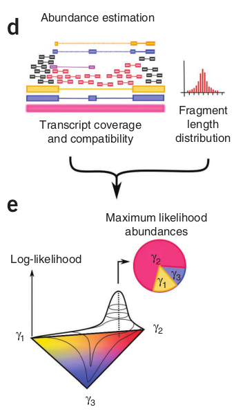1](cufflinks_1png.png)
---
### Cufflinks

![Cufflinks2](cufflinks_2png.png)

---
### Cufflinks

![Cufflinks3](cufflinks_3png.png)

---
### Cufflinks

![Cufflinks4](cufflinks_4png.png)

---
## Isoform analysis of RNA-seq data

### Software: MISO

Katz, Yarden, et al. "Analysis and design of RNA sequencing experiments for identifying isoform regulation." *Nature Methods* 7.12 (2010): 1009.

--
* Mixture of isoforms (MISO) using Bayesian inference

* Calculates the Percentage Spliced In (PSI or `$\Psi$`) reads for each transcript or splice junction

* Rescales `$\Psi$` based on library size and number of mapped reads

* Generates Sashimi plots

* Can perform a comparison of two conditions, but cannot account for covariates or multiple comparisons

* Does not model biological variability

---
### MISO algorithm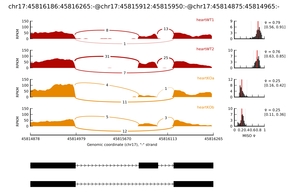

---
### Sashimi plots

![Sashimi plot](sashimiPlot.png)
---
### Example of a MISO pipeline

<div id="htmlwidget-26409803783642e5560f" style="width:504px;height:600px;" class="grViz html-widget"></div>
<script type="application/json" data-for="htmlwidget-26409803783642e5560f">{"x":{"diagram":"\ndigraph boxes_and_circles {\n\n  # a \"graph\" statement\n  graph [overlap = true, fontsize = 10]\n\n  # several \"node\" statements\n  node [shape = box,\n        fontname = Helvetica]\n  FASTQT; FASTQN; GFF; BAMT; BAMN; MISOT; MISON; DifferentialIsoforms\n\n  node [shape = circle,\n        fixedsize = false,\n        width = 1] // sets as circles\n  STAR; MISORUN; MISOCOMPARE;\n\n  # several \"edge\" statements\n  FASTQT->STAR STAR->BAMT\n  FASTQN->STAR STAR->BAMN\n  GFF->MISORUN BAMT->MISORUN BAMN->MISORUN\n  MISORUN->MISOT MISORUN->MISON\n  MISOT->MISOCOMPARE MISON->MISOCOMPARE\n  MISOCOMPARE->DifferentialIsoforms\n}\n","config":{"engine":"dot","options":null}},"evals":[],"jsHooks":[]}</script>

---
### Software: DEXSeq

Anders, Simon, Alejandro Reyes, and Wolfgang Huber. "Detecting differential usage of exons from RNA-seq data." *Genome Research* 22.10 (2012): 2008-2017.

--
Fits one model per gene (similar to DESeq), with two additional parameters:

--
* One with dimension `$l$` accounting for the fraction of reads mapping to `$l$` different bins

--
* One additional parameter of `$l$` dimensions accounting for the effect of condition on fraction of reads in each bin

---

### DEXSeq plot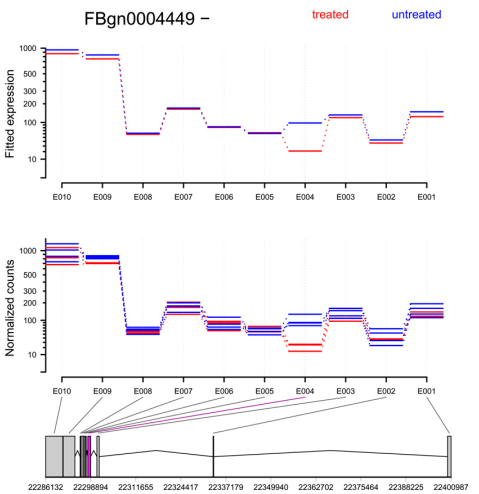

![DEXSeq plot](DexSeqPlot.png)

---
## DEXseq pipeline
<div id="htmlwidget-8ba44c6dd524b600429b" style="width:504px;height:600px;" class="grViz html-widget"></div>
<script type="application/json" data-for="htmlwidget-8ba44c6dd524b600429b">{"x":{"diagram":"\ndigraph boxes_and_circles {\n\n  # a \"graph\" statement\n  graph [overlap = true, fontsize = 10]\n\n  # several \"node\" statements\n  node [shape = box,\n        fontname = Helvetica]\n  FASTQT; FASTQN; GFF; BAMT; BAMN; ExonCountsT; ExonCountsN; DifferentialIsoforms\n\n  node [shape = circle,\n        fixedsize = false,\n        width = 1] // sets as circles\n  STAR; HTSeq; DEXSeq;\n\n  # several \"edge\" statements\n  FASTQT->STAR STAR->BAMT\n  FASTQN->STAR STAR->BAMN\n  GFF->HTSeq\n  GFF->DEXSeq BAMT->HTSeq BAMN->HTSeq\n  HTSeq->ExonCountsT HTSeq->ExonCountsN\n  ExonCountsT->DEXSeq ExonCountsN->DEXSeq\n  DEXSeq->DifferentialIsoforms\n}\n","config":{"engine":"dot","options":null}},"evals":[],"jsHooks":[]}</script>
---
## What is the advantage of each tool?

<table class="table table-striped" style="font-size: 9px; width: auto !important; float: left; margin-right: 10px;">
 <thead>
  <tr>
   <th style="text-align:left;"> Software </th>
   <th style="text-align:left;"> De novo isoform annotation </th>
   <th style="text-align:left;"> Pairwise comparison </th>
   <th style="text-align:left;"> Multiple replicates </th>
   <th style="text-align:left;"> Covariates </th>
   <th style="text-align:left;"> Uses splice junction information </th>
   <th style="text-align:left;"> Plotting </th>
   <th style="text-align:left;"> Usability </th>
  </tr>
 </thead>
<tbody>
  <tr>
   <td style="text-align:left;"> Cufflinks </td>
   <td style="text-align:left;"> Yes </td>
   <td style="text-align:left;"> No </td>
   <td style="text-align:left;"> No </td>
   <td style="text-align:left;"> No </td>
   <td style="text-align:left;"> Yes </td>
   <td style="text-align:left;"> No </td>
   <td style="text-align:left;"> Easy </td>
  </tr>
  <tr>
   <td style="text-align:left;"> MISO </td>
   <td style="text-align:left;"> No </td>
   <td style="text-align:left;"> Yes </td>
   <td style="text-align:left;"> No </td>
   <td style="text-align:left;"> No </td>
   <td style="text-align:left;"> Yes </td>
   <td style="text-align:left;"> Yes </td>
   <td style="text-align:left;"> Moderate </td>
  </tr>
  <tr>
   <td style="text-align:left;"> DEXSeq </td>
   <td style="text-align:left;"> No </td>
   <td style="text-align:left;"> Yes </td>
   <td style="text-align:left;"> Yes </td>
   <td style="text-align:left;"> Yes </td>
   <td style="text-align:left;"> No </td>
   <td style="text-align:left;"> Yes </td>
   <td style="text-align:left;"> Easy </td>
  </tr>
</tbody>
</table>

---
### Tutorial

Main task: Identify differentially expressed isoforms between breast tumour and normal lymphoblastoid controls

* Make MISO index

* Identify differential isoforms in MISO

* Make Sashimi plots

* Use HTSeq to obtain table of counts for DEXseq

* Run DEXseq and visualize the results

* Compare the results from MISO and DEXSeq

---
## Bash environmental variables

* In R, you could create variables and store strings, numbers, etc.

```r
## Example of a number
my_number = 42
## Example of a string
my_name = "Mehran"
## My document folder path
path_mydocs = "/home/mehran/Documents"
## Example of a vector of numbers
my_lucky_numbers = c(37, 42, 91)
## print my third lucky number
print(my_lucky_numbers[3])
```
---
### Variables in bash

* You could do the same in bash (convention is to use upper case)

```bash
## Example of a number
MUNUMBER=42
## Example of string
MYNAME=Mehran
## My document folder path
PATHMYDOC="/home/mehran/Documents"
## Example of a vector of numbers (aka array)
MYLUCKYNUMBERS=(37 42 91)
## print my third lucky number
echo ${MYLUCKYNUMBERS[2]}
## Print all my lucky numbers
echo ${MYLUCKYNUMBERS[@]}
```
---
## For loop in bash

* In R, you could iterate through elements of an array

```r
for(number in my_lucky_numbers){
  print(paste("One of my lucky numbers", number))
}
```

* You could do the same in bash with a different syntax

```bash
for NUMBER in ${MYLUCKYNUMBERS[@]}
do
  echo "One of my lucky numbers is $NUMBER"
done
```
---
### Operations on file paths

* Command line programs require positional as well as specific parameters

* mkdir program, for example, accepts a positional argument which is the name of the folder it wants to create

* mkdir also has specific and optional parameters you can learn about by doing

```bash
  mkdir --help
```

```bash
## Your scratch directory path on SciNet teach cluster is stored in $SCRATCH
echo $SCRATCH ## This gives you the full path to your scratch folder
## You can list the files and folders under each folder using ls
ls $SCRATCH
## ls also has an optional parameter -l which provides more information
ls -l $SCRATCH
## You can store all the files under a folder into an array
FILESINMYSCRATCH=($(ls $SCRATCH))
```

---
## Useful file operation commands

* In terminal, you are always located in some directory. you can see where you are using pwd (print working directory)

```bash
pwd
## Current directory is always also saved to $PWD
echo $PWD
```

* You can change your file path usind cd (change directory)

```bash
cd $SCRATCH
pwd
echo $PWD
```

---
## Indexing MISO

Task: Index the chromosome 22 with a proper GFF file

* Make a directory in your scratch called isoformAnalysis

```bash
mkdir $SCRATCH/isoformAnalysis
cd $SCRATCH/isoformAnalysis
```

* Under isoformAnalysis, make *datasets* and download chr22 GFF file there

```bash
mkdir $SCRATCH/isoformAnalysis/datasets
cd $SCRATCH/isoformAnalysis/datasets
wget ftp://ftp.ensembl.org/pub/release-95/gff3/homo_sapiens/Homo_sapiens.GRCh38.95.chromosome.22.gff3.gz
```

* The assmebly you are using uses *chr22* and not *22*. Change that in the gff file without compressing the output (MISO requires uncompressed gff). Hint: use a program called *sed*

```bash
# In sed, you can replace all occurences of a search (x) with any character (y): cat myfile | sed 's/x/y/g'
zcat Homo_sapiens.GRCh38.95.chromosome.22.gff3.gz | sed 's/^22/chr22/g' > Homo_sapiens.hg38.95.chromosome.22.gff3
```
---
### Indexing MISO

* Use index_gff in MISO binary folder and index the GFF under isoformAnalysis/datasets/misoIndex

```bash
# MISOBIN=/scinet/teach/software/2018a/opt/base/miso/0.5.4/bin
# export PATH="$MISOBIN":$PATH
module load anaconda2 miso

MISOINDEX=$SCRATCH/isoformAnalysis/datasets/misoIndex
GFF=$SCRATCH/isoformAnalysis/datasets/Homo_sapiens.hg38.95.chromosome.22.gff3
mkdir $MISOINDEX
index_gff --index $GFF $MISOINDEX
```

---
## Run MISO -- individual files

* Run MISO individually for each of the sorted bam files.
  * You can use for loops to repeat the same instructions for several files

* Save the output to isoformAnalysis/misoRuns in your scratch directory

```bash
MISOINDEX=$SCRATCH/isoformAnalysis/datasets/misoIndex
BAMDIR=/scratch/j/johanna/johanna/ISOFORM_TUTORIAL/BAMS
BAMFILES=($(ls $BAMDIR | grep .bam | grep -v bam.bai))
OUTMAIN=$SCRATCH/isoformAnalysis/misoRuns
mkdir $OUTMAIN
```
---

---

```bash
for BAMFILE in ${BAMFILES[@]}
do
  # Using sed to remove extension for creating the output folder
  SAMPLENAME=$(echo $BAMFILE | sed 's/.bam//')
  # Create the environmental variable OUTDIR for saving miso output to
  OUTDIR=$OUTMAIN/$SAMPLENAME
  # Create the folder with the value saved into environmental variable $OUTDIR
  mkdir -p $OUTDIR
  # Print to the screen which bam file is currently being used
  echo "Running MISO for $BAMFILE"
  # Run miso
  miso --run $MISOINDEX $BAMDIR/$BAMFILE --output-dir $OUTDIR/ --read-len 150
  # Print summary to the screen
  echo "Summarizing MISO for $BAMFILE"
  # Run MISO summary
  summarize_miso --summarize-samples $OUTDIR $OUTDIR
done
```

---
## Run MISO -- comparison mode

* Compare the first biological replicate of breast cancer with the first biological replicate of lymphoblastoid cells in MISO comparison mode

```bash
MISODIR=$SCRATCH/isoformAnalysis/misoRuns
TUMOUR=$MISODIR/hcc1395_tumor_rep1_sorted
NORMAL=$MISODIR/hcc1395_normal_rep1_sorted
OUTDIR=$MISODIR/ComparisonRep1
mkdir $OUTDIR
compare_miso --compare-samples $TUMOUR $NORMAL $OUTDIR
```
---
### Select top hits from MISO comparison mode

* Open the miso_bf file in R

* Add a new column which has the most extreme value in the bayes_factor column

* Add a new column which has the most extreme value in the diff column

```bash
module load gcc anaconda2 dexseq
R
```

---

```r
miso_df = read.csv(
  "hcc1395_tumor_rep1_sorted_vs_hcc1395_normal_rep1_sorted.miso_bf", header=T, sep="\t")
head(miso_df, 1)
miso_df$MostExtremeBF = sapply(as.character(miso_df$bayes_factor), function(x){
  bayes_factors = as.numeric(unlist(strsplit(x, ",", T)))
  return(max(bayes_factors))
})
miso_df$MostExtremeDiff = sapply(as.character(miso_df$diff), function(x){
  bayes_factors = as.numeric(unlist(strsplit(x, ",", T)))
  return(max(abs(bayes_factors)))
})
```

---
## Visualize results with MISO Sashimi script

MISO requires a setting file for making a sashimi plot.
The setting file requires to know:

* Width, height, font size, resolution, color, etc.

* Path to each BAM file

* Coverage of each bam file

* Full path to each bam file

* Name to use for each bam file

* You can create a file named *miso_setting.txt* with nano and copy the contents of next slide to it

```bash
cd $SCRATCH/isoformAnalysis
nano miso_setting.txt
# <Paste>
# <Ctrl + X> to save and exit
```

---

```python
[data]
bam_prefix = /scratch/t/teachmmg3003/mmg3003ta002/BAMS
miso_prefix = /scratch/t/teachmmg3003/mmg3003ta002/isoformAnalysis/misoRuns
bam_files = ["hcc1395_tumor_rep1_sorted.bam", "hcc1395_normal_rep1_sorted.bam"]
miso_files = ["hcc1395_tumor_rep1_sorted", "hcc1395_normal_rep1_sorted"]
[plotting]
fig_width = 10
fig_height = 8
intron_scale = 50
exon_scale = 4
logged = True
font_size = 6.5
bar_posteriors = True
ymax = 150
nyticks = 3
nxticks = 4
show_ylabel = True
show_xlabel = True
show_posteriors = True
resolution = 0.5
posterior_bins = 40
gene_posterior_ratio = 5
colors = ["#FE9A2E", "#08088A"]
coverages = [100000, 110000]
bar_color = "b"
bf_thresholds = [0, 1, 2, 5, 10, 20]
```
---
### Sashimi plot with MISO

```bash
SETTINGFILE=$SCRATCH/isoformAnalysis/miso_setting.txt
OUTDIR=$SCRATCH/isoformAnalysis/sashimiPlots
sashimi_plot --plot-event "gene:ENSG00000197077" $MISOINDEX $SETTINGFILE --output-dir $OUTDIR
## Change the file name because it contains ":"
cd $SCRATCH/isoformAnalysis/sashimiPlots
mv "gene:ENSG00000197077.pdf" "ENSG00000197077.pdf"
```

---
### How to see a PDF file you created in the cluster?

* If the cluster supports graphic applications (allows X11 forwarding), you can use xdg-open

```bash
ssh -X user@server
cd $SCRATCH/isoformAnalysis/sashimiPlots
xdg-open "ENSG00000197077.pdf"
```

* Otherwise, transfer the files to your local computer

```bash
## Without ssh into cluster
scp user@server:$SCRATCH/isoformAnalysis/sashimiPlots/ENSG00000197077.pdf $PWD/Downloads
```

---
## Prepare the GFF file for DEXseq

Download the GRCh38 GTF file from Ensembl, filter for chr22, and convert it to a specific gff using DEXSeq-accompanied python script *dexseq_prepare_annotation.py*

```bash
cd $SCRATCH/isoformAnalysis/datasets
wget ftp://ftp.ensembl.org/pub/release-95/gtf/homo_sapiens/Homo_sapiens.GRCh38.95.gtf.gz
zcat Homo_sapiens.GRCh38.95.gtf.gz | sed 's/^/chr/g' | fgrep chr22 > chr22_Homo_sapiens.GRCh38.95.gtf

module load anaconda3/5.2.0
module load htseq/0.11.1
DEXSEQSCRIPTS=/scinet/teach/software/2018a/opt/gcc-7.3.0/dexseq/1.24.4/DEXSeq/python_scripts
python $DEXSEQSCRIPTS/dexseq_prepare_annotation.py chr22_Homo_sapiens.GRCh38.95.gtf chr22_Homo_sapiens.GRCh38.95.gff
```

---
## Use HTSeq to obtain read counts for each exon

DEXSeq has a python script which uses HTSeq for obtaining read counts for each exon.
It requires read-group sorted BAM files.

```bash
GFF=/scratch/j/johanna/johanna/ISOFORM_TUTORIAL/datasets/chr22_Homo_sapiens.GRCh38.95.gff
BAMDIR=/scratch/j/johanna/johanna/ISOFORM_TUTORIAL/BAMS
BAMFILES=($(ls $BAMDIR | grep .bam | grep -v bam.bai))
OUTMAIN=$SCRATCH/isoformAnalysis/DexSeqCounts
mkdir $OUTMAIN
for BAMFILE in ${BAMFILES[@]}
do
  SAMPLENAME=$(echo $BAMFILE | sed 's/.bam//')

echo "Running MISO for $BAMFILE"
  python $DEXSEQSCRIPTS/dexseq_count.py -r pos -p yes -f bam $GFF $BAMDIR/$BAMFILE $OUTMAIN/$SAMPLENAME\_DexSeqCount.tsv
done
```

---
## Identify genes with different transcripts using DEXseq

In R, load the files and identify genes with differential isoforms.

```bash
module load gcc anaconda2 dexseq
R
```

---

```r
options(stringsAsFactors=FALSE)
require(DEXSeq)

## Set input/output information
scratch_dir = Sys.getenv("SCRATCH")
johanna_dir = "/scratch/j/johanna/johanna/ISOFORM_TUTORIAL"
gffPath = file.path(johanna_dir, "datasets", "chr22_Homo_sapiens.GRCh38.95.gff")
outDir = file.path(scratch_dir, "isoformAnalysis",
                   "dexSeqOutput")
dir.create(outDir)
countDir = file.path(johanna_dir, #"isoformAnalysis",
                     "DexSeqCounts")

## Get full path of count.tsv files
conditions = character()
countFiles = dir(countDir)[grep("DexSeqCount.tsv", dir(countDir))]
for(countFile in countFiles){
  name_parts = unlist(strsplit(countFile, "_", T))
  conditions = c(conditions, name_parts[2])
}
print(countFiles)
```
---
## Run DEXSeq commands

DEXSeq needs to know the full path to each of the DEXSeq count file, and how to treat them in a statistical model.
The statistical model of DEXSeq can handle is a generalized linear model and can handle any type of comparison a GLM can.

```r
setwd(countDir)
sampleTable = data.frame(condition=conditions,
                         libType="paired-end")
rownames(sampleTable) = basename(countFiles)
dxd = DEXSeqDataSetFromHTSeq(
    countFiles, sampleData=sampleTable,
    design= ~ sample + exon + condition:exon,
    flattenedfile=gffPath)

count_df = counts(dxd)
write.table(count_df, file=sprintf("%s/CountOfExons.tsv", outDir),
            quote=F, row.names=TRUE, sep="\t")
```
---
## Cont'd

```r
dxd = estimateSizeFactors(dxd)
dxd = estimateDispersions(dxd)
png(sprintf("%s/DispersionEstimate.png", outDir),
    width=7*200, height=7*200, res=200)
plotDispEsts(dxd)
dev.off()

dxd = testForDEU(dxd)
dxd = estimateExonFoldChanges( dxd, fitExpToVar="condition")
dxr1 = DEXSeqResults( dxd )
dxr_df = as.data.frame(dxr1)
write.table(dxr_df, file=sprintf("%s/DifferentialExonUsage.tsv", outDir),
            quote=F, row.names=TRUE, sep="\t")

save(list="dxd",
     file=sprintf("%s/DEXSEQ-OBJ.RDATA", outDir),
     compression_level=9, compress="xz")
```
---
## Visualize with DEXSeq

Visualize the top 10 genes with the highest test statistic which have adjusted p-value of less than 0.001

```r
dxr_df_sig = dxr_df[!is.na(dxr_df$padj) & dxr_df$padj < 0.001, ]
dxr_df_sig = dxr_df_sig[order(dxr_df_sig$stat, decreasing=TRUE), ]
dxr_df_sig = dxr_df_sig[nchar(rownames(dxr_df_sig)) < 30, ]

for(i in 1:10){
    gene_name = dxr_df_sig$groupID[i]
    pdf(sprintf("%s/%s_ExonUsagePlot.pdf", outDir, gene_name), 15, 15)
    plotDEXSeq(dxr1, gene_name, legend=TRUE, cex.axis=1.2, cex=1.3, lwd=2, displayTranscripts=TRUE)
    dev.off()
}
```
---
* Using UpSet plots for showing intersections

```r
require(UpSetR)
mutations = read.csv(system.file("extdata", "mutations.csv", package = "UpSetR"), header=T, sep = ",")
kable(mutations[1:8, 1:12]) %>% kable_styling(bootstrap_options = "striped", full_width = T, position = "float_left", font_size = 12)
```

<table class="table table-striped" style="font-size: 12px; float: left; margin-right: 10px;">
 <thead>
  <tr>
   <th style="text-align:left;"> Identifier </th>
   <th style="text-align:right;"> TTN </th>
   <th style="text-align:right;"> PTEN </th>
   <th style="text-align:right;"> TP53 </th>
   <th style="text-align:right;"> EGFR </th>
   <th style="text-align:right;"> MUC16 </th>
   <th style="text-align:right;"> FLG </th>
   <th style="text-align:right;"> RYR2 </th>
   <th style="text-align:right;"> PCLO </th>
   <th style="text-align:right;"> PIK3R1 </th>
   <th style="text-align:right;"> PIK3CA </th>
   <th style="text-align:right;"> NF1 </th>
  </tr>
 </thead>
<tbody>
  <tr>
   <td style="text-align:left;"> 02-0003 </td>
   <td style="text-align:right;"> 0 </td>
   <td style="text-align:right;"> 0 </td>
   <td style="text-align:right;"> 1 </td>
   <td style="text-align:right;"> 1 </td>
   <td style="text-align:right;"> 0 </td>
   <td style="text-align:right;"> 0 </td>
   <td style="text-align:right;"> 0 </td>
   <td style="text-align:right;"> 0 </td>
   <td style="text-align:right;"> 1 </td>
   <td style="text-align:right;"> 0 </td>
   <td style="text-align:right;"> 0 </td>
  </tr>
  <tr>
   <td style="text-align:left;"> 02-0033 </td>
   <td style="text-align:right;"> 0 </td>
   <td style="text-align:right;"> 0 </td>
   <td style="text-align:right;"> 1 </td>
   <td style="text-align:right;"> 0 </td>
   <td style="text-align:right;"> 0 </td>
   <td style="text-align:right;"> 0 </td>
   <td style="text-align:right;"> 0 </td>
   <td style="text-align:right;"> 0 </td>
   <td style="text-align:right;"> 0 </td>
   <td style="text-align:right;"> 1 </td>
   <td style="text-align:right;"> 1 </td>
  </tr>
  <tr>
   <td style="text-align:left;"> 02-0047 </td>
   <td style="text-align:right;"> 0 </td>
   <td style="text-align:right;"> 0 </td>
   <td style="text-align:right;"> 0 </td>
   <td style="text-align:right;"> 0 </td>
   <td style="text-align:right;"> 0 </td>
   <td style="text-align:right;"> 0 </td>
   <td style="text-align:right;"> 1 </td>
   <td style="text-align:right;"> 0 </td>
   <td style="text-align:right;"> 0 </td>
   <td style="text-align:right;"> 1 </td>
   <td style="text-align:right;"> 0 </td>
  </tr>
  <tr>
   <td style="text-align:left;"> 02-0055 </td>
   <td style="text-align:right;"> 1 </td>
   <td style="text-align:right;"> 1 </td>
   <td style="text-align:right;"> 1 </td>
   <td style="text-align:right;"> 0 </td>
   <td style="text-align:right;"> 0 </td>
   <td style="text-align:right;"> 0 </td>
   <td style="text-align:right;"> 0 </td>
   <td style="text-align:right;"> 0 </td>
   <td style="text-align:right;"> 0 </td>
   <td style="text-align:right;"> 0 </td>
   <td style="text-align:right;"> 0 </td>
  </tr>
  <tr>
   <td style="text-align:left;"> 02-2470 </td>
   <td style="text-align:right;"> 0 </td>
   <td style="text-align:right;"> 1 </td>
   <td style="text-align:right;"> 0 </td>
   <td style="text-align:right;"> 0 </td>
   <td style="text-align:right;"> 0 </td>
   <td style="text-align:right;"> 0 </td>
   <td style="text-align:right;"> 1 </td>
   <td style="text-align:right;"> 0 </td>
   <td style="text-align:right;"> 0 </td>
   <td style="text-align:right;"> 0 </td>
   <td style="text-align:right;"> 0 </td>
  </tr>
  <tr>
   <td style="text-align:left;"> 02-2483 </td>
   <td style="text-align:right;"> 0 </td>
   <td style="text-align:right;"> 0 </td>
   <td style="text-align:right;"> 1 </td>
   <td style="text-align:right;"> 0 </td>
   <td style="text-align:right;"> 0 </td>
   <td style="text-align:right;"> 0 </td>
   <td style="text-align:right;"> 0 </td>
   <td style="text-align:right;"> 1 </td>
   <td style="text-align:right;"> 0 </td>
   <td style="text-align:right;"> 0 </td>
   <td style="text-align:right;"> 0 </td>
  </tr>
  <tr>
   <td style="text-align:left;"> 02-2485 </td>
   <td style="text-align:right;"> 0 </td>
   <td style="text-align:right;"> 0 </td>
   <td style="text-align:right;"> 1 </td>
   <td style="text-align:right;"> 1 </td>
   <td style="text-align:right;"> 1 </td>
   <td style="text-align:right;"> 1 </td>
   <td style="text-align:right;"> 0 </td>
   <td style="text-align:right;"> 0 </td>
   <td style="text-align:right;"> 0 </td>
   <td style="text-align:right;"> 1 </td>
   <td style="text-align:right;"> 0 </td>
  </tr>
  <tr>
   <td style="text-align:left;"> 02-2486 </td>
   <td style="text-align:right;"> 0 </td>
   <td style="text-align:right;"> 0 </td>
   <td style="text-align:right;"> 0 </td>
   <td style="text-align:right;"> 0 </td>
   <td style="text-align:right;"> 0 </td>
   <td style="text-align:right;"> 0 </td>
   <td style="text-align:right;"> 0 </td>
   <td style="text-align:right;"> 0 </td>
   <td style="text-align:right;"> 0 </td>
   <td style="text-align:right;"> 0 </td>
   <td style="text-align:right;"> 0 </td>
  </tr>
</tbody>
</table>
---

```r
upset(mutations, sets = c("PTEN", "TP53", "EGFR", "PIK3R1", "RB1"),
      sets.bar.color = "#56B4E9",
      order.by = "freq", empty.intersections = "on")
```

---
## Home assignment (not final)

* Did you identify the same set of genes using MISO and DEXSeq?

* Use [UpSet plot](https://cran.r-project.org/web/packages/UpSetR/README.html) to show the number of transcripts found only by one method or with both methods.

* What could be the reason you find some genes with MISO but not with DEXSeq (and vice versa)?

* You might find some genes with DEXSeq but not with MISO. Why do you think this happens?

* You are working in a clinical research lab and present your findings to the lab director. After seeing your findings, the director is excited, but concerned that some of the genes you found when comparing differential isoforms in breast tumour and normal lymphoblasts might not be related to cancer.
  * What additional experiments would you perform and which software (MISO or DEXSeq) would you choose to address the lab director's concern?

---
### Home assignment (not final)

* You are reporting to director of a clinical research lab which doesn't know anything about the importance of alternative splicing. In the first page of the report:

* describe why studying isoforms is important
  
  * choose one software and describe how the software you chose investigates isoforms

* Based on the software you chose, sort the genes based on a measurement (or a mix of measurements) that gives you the genes with the most extreme changes in isoform in comparison of breast cancer cell line with lymphastoid cell line

* List the HUGO gene symbol for the top 10 genes based on the measurement you chose

* Include one plot for each gene and describe your findings from the plot (e.g. Gene X has alternative splicing of exon 7 or Gene Y has no clear alternative splicing pattern when we visually compare replicate 1 of each condition, etc.)

---